I was inspired by Damie Pak’s delightful work on a depiction of the Clair Obscure: Expedition 33 gommage if it happened in Boston. (By “inspired” I mean literally dared to try it by Damie, which, okay, was awesome.) It’s a really tremendous game with some of my favorite narrative elements and dialog cut-scenes in a game in a very long time. So it’s great fun to have a data project centered on the game’s gommage.

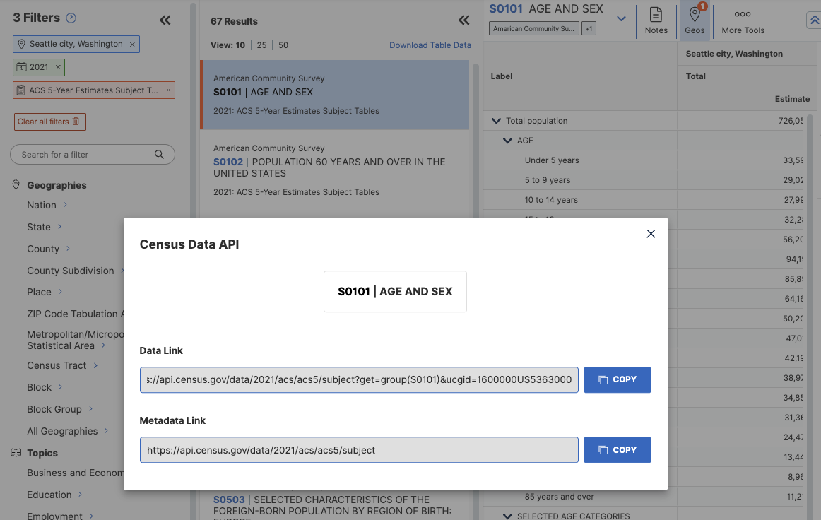
Damie did her project for Boston. Via Seattle’s (very good) city data site I hopped over to the narrative profile page for Seattle at the U. S. Census, where I found a table of population by age groups in the 2021 American Community Survey.
The Census web site has great tools for finding and interacting with your data. While surfacing an API call directly to the current view is a click away, the return of that request is a little tricky to deal with.
One could copy that URL offered by the Census, retrieve it via a request built with httr2, and see what the response looks like after a little bit of transformation, as I do here:
census_url <- "https://api.census.gov/data/2021/acs/acs5/subject?get=group%28S0101%29&for=S0101_C01_002E%2CS0101_C01_003E%2CS0101_C01_004E%2CS0101_C01_005E%2CS0101_C01_006E%2CS0101_C01_007E%2CS0101_C01_008E%2CS0101_C01_009E%2CS0101_C01_010E%2CS0101_C01_011E%2CS0101_C01_012E%2CS0101_C01_013E%2CS0101_C01_014E%2CS0101_C01_015E%2CS0101_C01_016E%2CS0101_C01_017E%2CS0101_C01_018E%2CS0101_C01_019E&&ucgid=1600000US5363000"

req <- request(census_url)
resp <- req_perform(req)

df <- resp |>
  resp_body_string() |>
  jsonlite::fromJSON() |>
  as_tibble()
names(df) <- as.character(df[1,])
df[2,] |>
  select(GEO_ID, NAME, starts_with("S0101_C01_00")) |>
  pivot_longer(cols=everything())
# A tibble: 38 × 2
name value
<chr> <chr>
1 GEO_ID 1600000US5363000
2 NAME Seattle city, Washington
3 S0101_C01_001E 726054
4 S0101_C01_001EA <NA>
5 S0101_C01_001M 87
6 S0101_C01_001MA <NA>
7 S0101_C01_002E 33592
8 S0101_C01_002EA <NA>
9 S0101_C01_002M 1380
10 S0101_C01_002MA <NA>
# ℹ 28 more rowsWith a little more screwing around, that’s a useful tibble of data: Those S0101 values are the population measures for the sum and then the individual age categories in the census data. S0101_C01_002E is the population in the 0-5 years age range, for example.
That effort is kind of a pain. And that’s where censusapi and tidycensus come to the rescue! Both packages provide methods to compose a request to the Census APIs and then helpfully shape the data returned from those requests.
~not pictured: a whole bunch of trial and error to figure out how to get what I need~
Huzzah! A request like this with the get_acs function in {tidycensus} will return a nice tibble of data from the ACS. This gets data for census-designated places in the ACS for the specified state. variables is a list I’m providing of all the S0101 data points:
fields <- c("S0101_C01_002E", "S0101_C01_003E", "S0101_C01_004E", "S0101_C01_005E", "S0101_C01_006E", "S0101_C01_007E", "S0101_C01_008E", "S0101_C01_009E", "S0101_C01_010E", "S0101_C01_011E", "S0101_C01_012E", "S0101_C01_013E", "S0101_C01_014E", "S0101_C01_015E", "S0101_C01_016E", "S0101_C01_017E", "S0101_C01_018E", "S0101_C01_019E")
get_acs(
    geography = "place",
    state = "WA",
    variables = fields,
    year = 2021, show_call=TRUE)
# A tibble: 11,502 × 5
GEOID NAME variable estimate moe
<chr> <chr> <chr> <dbl> <dbl>
1 5300100 Aberdeen city, Washington S0101_C01_002 1365 267
2 5300100 Aberdeen city, Washington S0101_C01_003 1325 335
3 5300100 Aberdeen city, Washington S0101_C01_004 1340 302
4 5300100 Aberdeen city, Washington S0101_C01_005 1469 256
5 5300100 Aberdeen city, Washington S0101_C01_006 842 249
6 5300100 Aberdeen city, Washington S0101_C01_007 895 210
7 5300100 Aberdeen city, Washington S0101_C01_008 1026 189
8 5300100 Aberdeen city, Washington S0101_C01_009 1271 238
9 5300100 Aberdeen city, Washington S0101_C01_010 1178 246
10 5300100 Aberdeen city, Washington S0101_C01_011 881 166
# ℹ 11,492 more rowsAfter spending some time sorting out the method, I packaged all the work into a function to retrieve the data and then process the gommage years for a specified place. I took for granted the assumptions that Damie made, such as no new births taking place and gommage being the only thing that would remove anybody from the population.
Code
gommage_place_data <- function(city=NULL,
state=NULL,
abbrev=NULL) {
if (is.null(city)| is.null(state) | is.null(abbrev)) {
stop("city, state, and abbrev for state must be specified")
}
census_age_labels <-
tibble(
code = c(
"S0101_C01_002E", "S0101_C01_003E", "S0101_C01_004E", "S0101_C01_005E", "S0101_C01_006E", "S0101_C01_007E", "S0101_C01_008E", "S0101_C01_009E", "S0101_C01_010E", "S0101_C01_011E", "S0101_C01_012E", "S0101_C01_013E", "S0101_C01_014E", "S0101_C01_015E", "S0101_C01_016E", "S0101_C01_017E", "S0101_C01_018E", "S0101_C01_019E"),
under = c(5, 10, 15, 20, 25, 30, 35, 40, 45, 50, 55, 60, 65, 70, 75, 80, 85, 100),
over = c(0, 5, 10, 15, 20, 25, 30, 35, 40, 45, 50, 55, 60, 65, 70, 75, 80, 85)) |>
mutate(match_label = substring(code, 1, 13))
populations <- get_acs(
geography = "place",
state = abbrev,
variables = census_age_labels$code,
year = 2021, show_call=TRUE)
city_pop <-
populations |>
filter(NAME == glue::glue("{city} city, {state}")) |>
left_join(census_age_labels,
join_by("variable"=="match_label"))
city_df <- city_pop |>
rowwise() |>
mutate(
dist = list(round(runif(estimate,
min=0,
max=under-over-1)))
)
city_df |>
unnest_auto(dist) |>
group_by(variable, estimate, dist, under, over) |>
tally() |>
mutate(city = city,
age = over+dist,
gyear = round((100-age)/2)) |>
arrange(age)
}- 1
- this tibble aligns the returned census variables with the low and high age ranges for each category, and sets us up to join with the API tibble
- 2
-
request data using the Census API and tidycensus
- 3
- make a distribution of ages in each age range, and save as a list to each row
- 4
- unnest_auto expands the age distribution from a list into new rows for each record. We tally them for each discrete age — that provides the total number of people of each estimated age — and can then calculate the age of gommage for each age group (thanks to Damie’s math!)
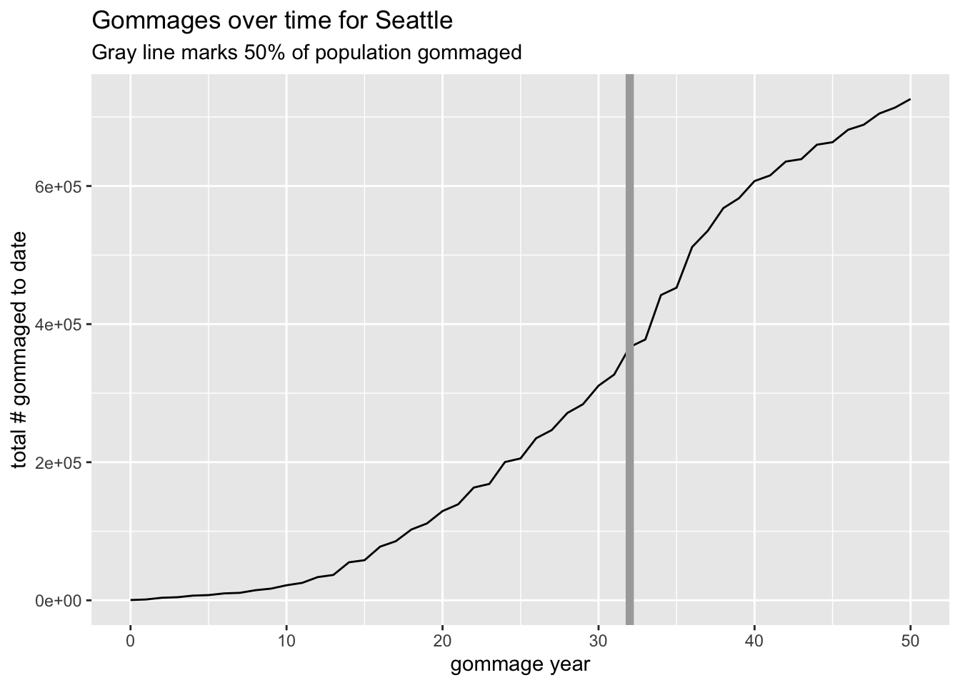
I also make functions to build a bar plot of the gommages by year, and a plot of the cumulative number of gommages over time.
Code
barplot_gommage <- function(gommage=NULL, highlight=NULL) {
    # highlight is optional current age for which
    # to draw focal gommage year

    if (is.null(gommage)) {
        stop("must specify gommage data set")
    }

   city <- gommage$city[1]
   p <- gommage |>
    ggplot(aes(x=gyear, y=n)) +
    geom_bar(stat = "identity") +
    labs(x="year of gommage", y="",
    title = glue::glue("{city} gets gommaged"),
    subtitle = "Number of people gommaged per year until everybody is gone")
    if(!is.null(highlight)) {
        g_highlight = round((100-highlight)/2)
        p + geom_vline(xintercept=g_highlight,
          color="red",
          size=2) +
        labs(caption = glue::glue("Red line marks gommage year for current age {highlight}"))
    } else {
        p
    }
}

cumulative_gommage_plot <- function(gommage) {
  if(is.null(gommage)) {
    stop("must specify gommage data set")
  }

  city <- gommage$city[1]
  cumulative_gommage <- gommage |>
      ungroup() |>
      summarise(.by=gyear, total=sum(n)) |>
      arrange(gyear) |>
      mutate(cs = cumsum(total),
        grand_total = sum(total),
        half = grand_total/2,
        diff = cs-half)

  halfway <- cumulative_gommage |> filter(diff > 0) |> slice(1)

  cumulative_gommage |>
      ggplot(aes(x=gyear, y=cs)) +
      geom_line() +
      labs(x="gommage year",
        y="total # gommaged to date",
        title=glue::glue("Gommages over time for {city}"),
        subtitle = "Gray line marks 50% of population gommaged") +
      geom_vline(xintercept = halfway$gyear, size=2, color="darkgray")
}
Now (finally) I can use variations of each of those functions to build plots of gommages for interesting places.1
g <-
gommage_place_data(city="Seattle",
  state="Washington",
  abbrev = "WA")

g |> barplot_gommage(highlight=35)
g |> cumulative_gommage_plot()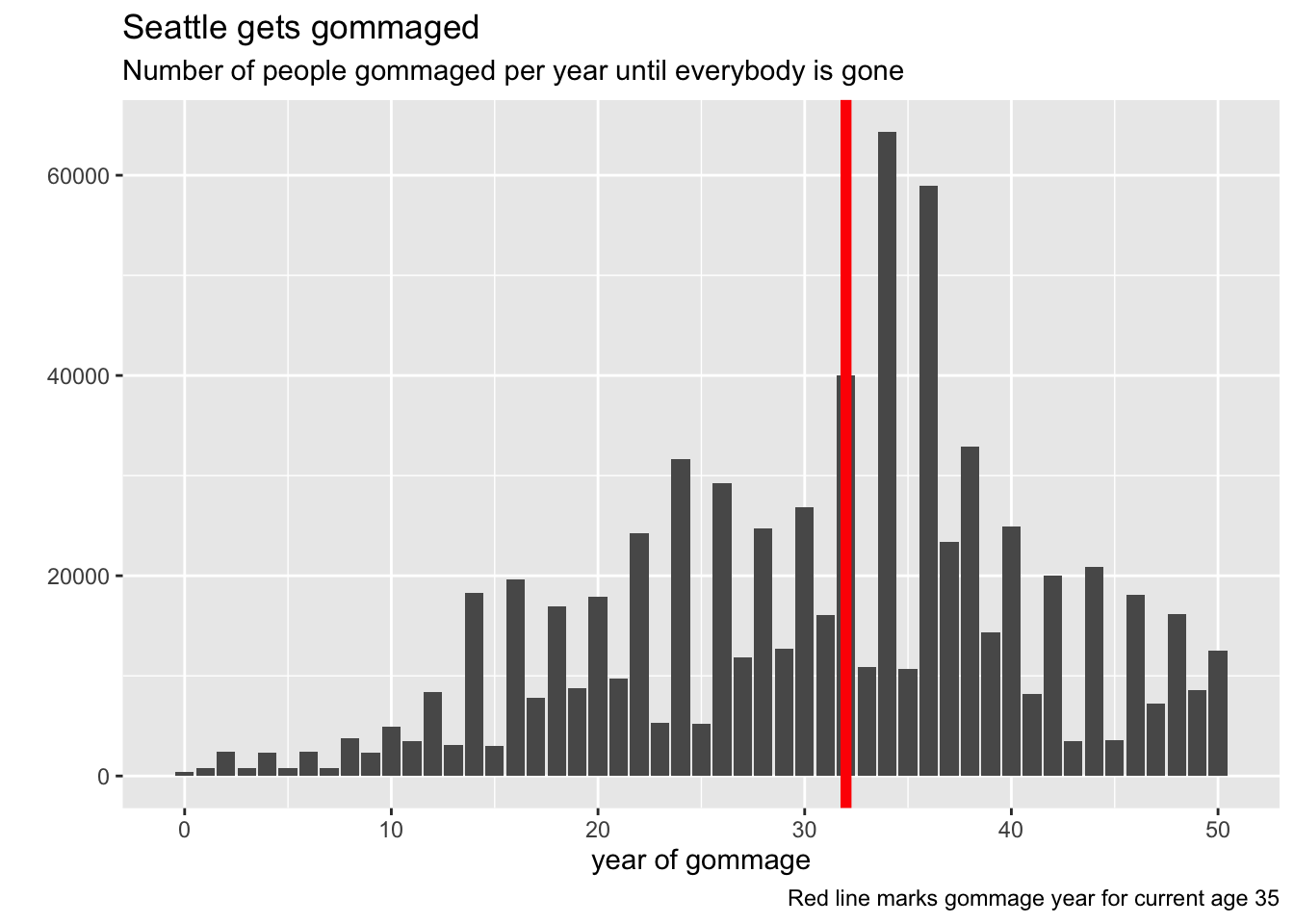
We can do Damie’s boston:
g <- gommage_place_data(city="Boston", state="Massachusetts", abbrev="MA")

g |> barplot_gommage(highlight=31)
g |> cumulative_gommage_plot()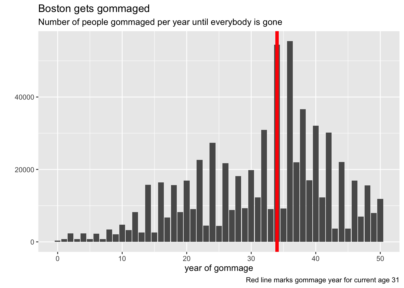

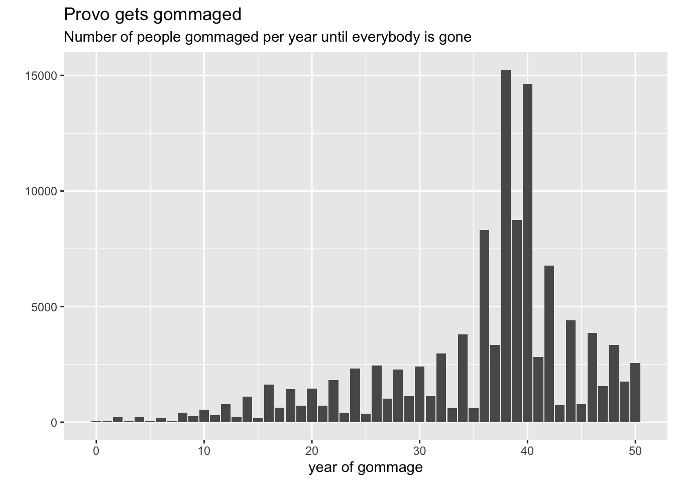
And it’s interesting to check out cities that tend towards much younger or older populations:
gommage_place_data(city="Lake Havasu City",
  state="Arizona", abbrev="AZ") |>
  barplot_gommage()
gommage_place_data(city="Provo",
  state="Utah", abbrev="UT") |>
  barplot_gommage()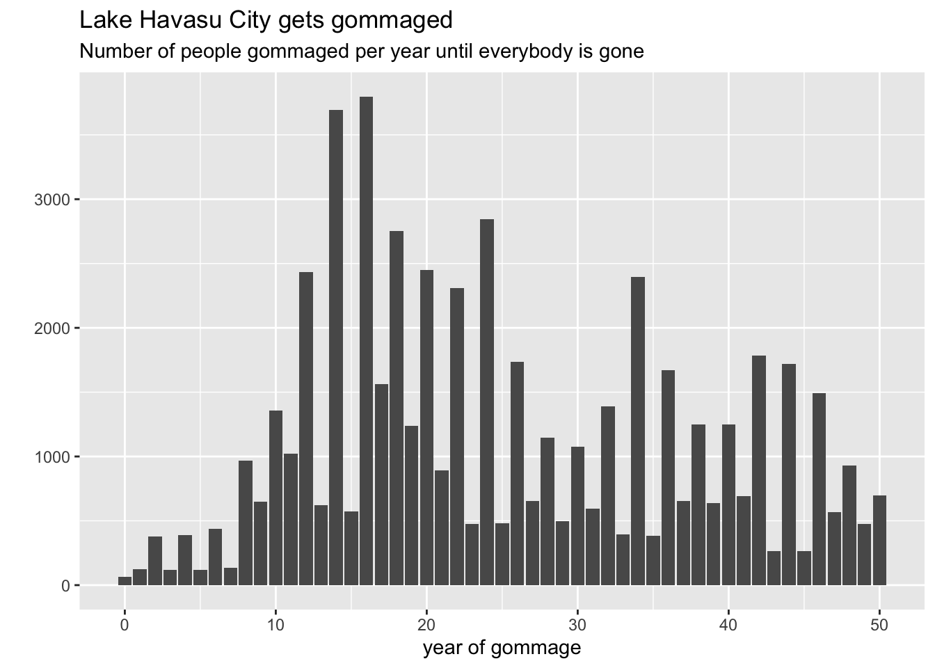
So there you have it! A reusable, reliable method for gommaging just about any city you want. Be your own Painttress! Thanks, Damie, for the motivation to go spelunking in the census and make something fun.